
Part 2 -- Arrays, Math, and Plotting in Python
Objectives
Here we will be exploring two external libraries in Python, NumPy (Numerical Python) and Matplotlib (a plotting library that uses a number of conventions common in MATLAB).
We will also revisit the strange element of Python indexing, which as we saw in the last session can be... perplexing - especially for people migrating from other languages.
Libraries in Python
Python is widely used and, as a consequence, it has accrued a large number of support libraries of functions and resources. Some are very highly specialized. Others are sufficiently generalized to have developed wide use. Some are also integerated into more specir
Today we will work with two libaries that are useful in general computation and in looking at those compitations.
- NumPy: a library that includes support for arrays, matrices, and high-level math functions.
- Matplotlib: a useful 2-d plotting library.
Calling the Libraries we'll use today
So, let's get started and load the libraries we will use today.
Notice the call to matplotlib (that's our graphing library). The pyplot is a sublibrary that emulates some handy Matlab plot functions. They are very popular in scientific Python use, and many libraries that do specialized work for a given discipline are built to leverage matplotlib.pyplot.
A common way to load libraries is to use the following format:
import *name of the libary* as *nickname for library*
##########################################################
#
# Library Calls.
#

import numpy             as np

import matplotlib.pyplot as plt

#
##########################################################
Kicking NumPy's Tires
Let's start small:
To invoke a one of these functionsm we need to use the identifier variable I declared above (i.e., np for NumPy). For example to calculate atan(1), we would do the following.
#############################################
#
# Calling a math function with NumPy...
#

x = 1.0

y = np.arctan(x)

print("atan(",x,") = ", y)

#
#############################################
atan( 1.0 ) = 0.7853981633974483
(which, if you remember, is a quarter of $\pi$)
Notice that we invoke the library and then the function. Here, the function is numpy.arctan. (For more "traditional" math functions, you can look here).
#############################################
#
# Making PI with NumPy
#


pi = 4 * np.arctan(x)

print("4 * atan(",x,") = ", pi)

#
#############################################
4 * atan( 1.0 ) = 3.141592653589793
(And while we're here -- and we're throwing the game given what we're trying to demonstrate here -- we also have some basic math constants that are available to us)
#############################################
#
# Calling PI and "e" as constants with NumPy
#

# pi

print("    numpy's constant pi = ", np.pi )

# e

print("numpy's constant exp(1) = ", np.exp(1), "or", np.e )

#
#############################################
    numpy's constant pi =  3.141592653589793
numpy's constant exp(1) =  2.718281828459045 or 2.718281828459045
Arrays in Python using NumPy
But here with NumPy, what we want to do is create an "empty" or "zero'ed" 1-d array (or "vector") to contain our answers to PI as calculated using various integrals of our above case example.
This example below uses a function called numpy.zeros(). Other functions used to make numpy arrays can be found here.
For example, let's make an empty array of 5 elements and populate them with zeros.
#############################################
#
# Create an vector 5-cells long and put zeros
#   in all the slots
#

mylist = [1,2,3]

print(3*mylist)

all_zeros = np.zeros(5)

print("This is an array of all zeros 5 elements long")
print("all_zeros =", all_zeros)

print(all_zeros + 3)

#
#############################################
[1, 2, 3, 1, 2, 3, 1, 2, 3]
This is an array of all zeros 5 elements long
all_zeros = [0. 0. 0. 0. 0.]
[3. 3. 3. 3. 3.]
We also can create an array that goes from one value to another in equal intervals with numpy.arange() (that's one R, "array range" or if you'd rather, "a range")
This is a variant of a more general python structure called a "range()" While a range creates a counting range that cannot be directly viewed (which is rather strange), numpy.arange() can be viewed as a ... well... as an full array.
(And while we're here, we index arrays in Python starting with 0.)
Also as before the example below creates an array from 1 to 20 (not 21).
############################################
#
# Create an vector 5 cells long and put a
#    consecutive range of integers in them
#

range_from_0_to_4 = range(0, 4+1)

print("               range_from_0_to_4 = ", range_from_0_to_4)
print("Third Value of range_from_0_to_4 = ", range_from_0_to_4[2])
print(" ")

array_from_0_to_4 =  np.arange(0, 4+1)    # <- Finish Me!

print("array_from_0_to_4 = ",array_from_0_to_4 )

# also now that we are working with indexes in arrays
#   as we learned with Mathcad, we might want to see
#   if indexing starts at 0 or 1.

# Spoilers: it's zero!

print("array_from_0_to_4[1] = ", array_from_0_to_4[1] )

print("array_from_0_to_4[0] = ", array_from_0_to_4[0] )

#  want to oull only the first three values from the array?

print("array_from_0_to_4[0:3] (first four?) = ", array_from_0_to_4[0:3+1])  # <- Finish Me!

#
#############################################
               range_from_0_to_4 =  range(0, 5)
Third Value of range_from_0_to_4 =  2

array_from_0_to_4 =  [0 1 2 3 4]
array_from_0_to_4[1] =  1
array_from_0_to_4[0] =  0
array_from_0_to_4[0:3] (first four?) =  [0 1 2 3]
INTERMISSION! A Deep-Dive on Arrays in Python (Do this on your own!) The Adventures of Inclusive vs Exclusive Indexing (Or where Dr C rage-quited when learning Python!)

[OK the above gif is more relevant when we start talking about data frames using the Pandas package.]
Continuing from last time, remember how when Python loops from 0 to N, it's looping from 0 to N-1?
When migrating from older languages like Fortran or C, you may be used to what is called inclusive indexing... because, for some reason, there wouldn't be a need to give such a thing specific adjective when you'd think that it wouldn't be so bloody obvious and intuitive to do it any other way.
But Oh No.........
Python, along with a couple of other newer languages, does something different...
Let's first borrow from a commonly used language like MATLAB, or R. (let's assume we start our indexing with 0 like Python does).
strawman := (/ 1, 2, 3, 4, 5 /)
Let's ask for the last two values... Normally, we would intuit that it'd be ...
print( strawman(3:4) )

(/ 4, 5 /)
Now, let's do the same thing in Python.
This time, we'll use the numpy.array function.
#############################################
#
# let's make a no-nonsense array from 0 to 4
#

strawman = np.array([0,1,2,3,4])

print('strawman[] =', strawman)

#
# and let's pull what we think should be the last two?
#

print('strawman[3:4] =', strawman[3:4])

#
#############################################
strawman[] = [0 1 2 3 4]
strawman[3:4] = [3]
Whaaaa?
OK, here is what is happening when "slicing," as it's called, an array in Python. Python does something that may be seen to be counterintuitive.
the first index that is requested list or array subset is inclusive
that means that what you ask for is what you get. You ask for the 0 index, or in this case, index #4 when starting at zero, you ask for "3" get that one.
But..
the closing index that is requested from a list or array subset is exclusive so when you ask for the subset ending at #5 from zero.. it gives you... #4 from zero. so if you want number #5 from zero, instead of typing "4", you type the next one... "5".
#############################################
#
# let's make a no-nonsense array
#

#
# so if you use the way we normally think about it...
#

print('strawman[3:4+1] =', strawman[3:4+1] )

# or

print('strawman[3: 5 ] =', strawman[3:5]  )

#
#############################################
strawman[3:4+1] = [3 4]
strawman[3: 5 ] = [3 4]
If you want to go from a array value 4 to the end of the array you could do this. This is similar to NCL... but as shown here if you look closer there is a lack of consistancy of you forget that the first value requested is "inclusive", the second requested is exclusive.
#############################################
#
# Playing with Indices
#

#
# let's try this with various styles of front-to-end notation.
#

print('strawman = ', strawman)

print()

print('strawman[  3: ] =',  strawman[ 3:  ]) # second to last their way
print('strawman[  3  ] =',  strawman[   3 ]) # second to last alone
print('strawman[  4  ] =',  strawman[   4 ]) # last alone (first request is inclusive)
print('strawman[  -2 ] =',  strawman[  -2 ]) # second from last
print('strawman[  -1 ] =',  strawman[ -1  ]) # first from last first request is inclusive
print('strawman[-2:-1] =',  strawman[-2:-1]) # the last value is exclusive
print('strawman[-2:  ] =',  strawman[-2:  ]) # how they want you to pull the last 2.
print('strawman[  :3 ] =',  strawman[  :3 ]) # this pulls the first three index (0-to-2).


#
#############################################
strawman =  [0 1 2 3 4]

strawman[  3: ] = [3 4]
strawman[  3  ] = 3
strawman[  4  ] = 4
strawman[  -2 ] = 3
strawman[  -1 ] = 4
strawman[-2:-1] = [3]
strawman[-2:  ] = [3 4]
strawman[  :3 ] = [0 1 2]
When you JFGI what why this is the case you get an argument from "elegance."
Whatever...

...but still. I prefer the following adage...
"Elegance is skin deep... but intuitive functionality is to the bone."
Back On Track: Loops!
OK, let's start talking about the structures we've had in the videos this week.
Starting with Loops, we have two species of loops.
- Counting Loops (The For Loop)
- Conditional Loops (The While Loop)
The Counting Loops
Counting Loops leverage Ranges, which, as we saw above, have that inclusive exclusive pairing.
A few things.
- The Loops (and If-Elif-Else Blocks) start with: at the end of the starter line.
- You must then indent (Jupyter will do it for you).
- When done with the indent, the "cue" that you are out of the structure is simply returning to the previous indent level (or hard against the left margin). You'll see a nested system shortly.
Otherwise, we'll remember our session with Nanny (or, in this case, The Count from Sesame Street). Here, we will loop through a series of numbers starting at zero and ending at 10 - otherwise known as 11-minus-one (remember, the last index is exclusive).
To create our "range" of counting loop values, we'll be using the range() function/class.
#############################################
#
# Counting from Zero to Ten like The Count!
#

# <- Do Me!

print("my range : ", range(0,11) )

for i in range(0, 10+1):
    print(i, "  Mwaah!  Ha! Ha! Ha!")

print(" ")
print("**Thunder Clap**")


#
#############################################
my range :  range(0, 11)
0   Mwaah!  Ha! Ha! Ha!
1   Mwaah!  Ha! Ha! Ha!
2   Mwaah!  Ha! Ha! Ha!
3   Mwaah!  Ha! Ha! Ha!
4   Mwaah!  Ha! Ha! Ha!
5   Mwaah!  Ha! Ha! Ha!
6   Mwaah!  Ha! Ha! Ha!
7   Mwaah!  Ha! Ha! Ha!
8   Mwaah!  Ha! Ha! Ha!
9   Mwaah!  Ha! Ha! Ha!
10   Mwaah!  Ha! Ha! Ha!

**Thunder Clap**

Fun Fact. If that failure for the columns to align in the above output drives you as crazy as it does to me, there is a cute trick here, and I have to do this a lot in writing strings for file names:
- Convert the number to a string with the intrinsic str() function
- You can tack a command for the string to pad the string with zeros ("z"'s) with zeros with str.zfill()
#############################################
#
# Counting from Zero-Zero to Ten!
#

print(" ")

for i in range(0, 10+1):
    print(str(i).zfill(2), "  Mwaah!  Ha! Ha! Ha!")

print(" ")
print("**Another Thunder Clap, But This Time Nicely Aligned since The Count, like your prof, has OCD **")


#
#############################################
00   Mwaah!  Ha! Ha! Ha!
01   Mwaah!  Ha! Ha! Ha!
02   Mwaah!  Ha! Ha! Ha!
03   Mwaah!  Ha! Ha! Ha!
04   Mwaah!  Ha! Ha! Ha!
05   Mwaah!  Ha! Ha! Ha!
06   Mwaah!  Ha! Ha! Ha!
07   Mwaah!  Ha! Ha! Ha!
08   Mwaah!  Ha! Ha! Ha!
09   Mwaah!  Ha! Ha! Ha!
10   Mwaah!  Ha! Ha! Ha!

**Another Thunder Clap, But This Time Nicely Aligned since The Count, like your prof, has OCD **
You can also loop through an arbitrary list.

#####################################################
#
# For Looping through a List
#
#   notice that continuation is just starting a new
#      line like you can do in R
#

mousekateers = ["Sharon",
                 "Bobby",
                 "Lonnie",
                 "Tommy",
                 "Annette",
                 "Darlene",
                 "Cubby",
                 "Karen",
                 "Doreen"]


print("Roll Call!")


# <- Do Me!

for mousekateer in mousekateers:
    print(mousekateer + "!")

#
#####################################################
Roll Call!
Sharon!
Bobby!
Lonnie!
Tommy!
Annette!
Darlene!
Cubby!
Karen!
Doreen!
Conditional Loops (The While Loop)
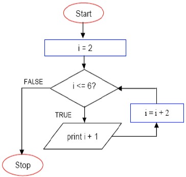
This one drops out when the condition is satisfied (this is what we used when we programmed Roots in Mathcad)
And let's do a revisit to our first foray into programming!
#####################################################
#
# While Loop (using our first loop EVER!)
#

# <- Do Me!

i = 2

while (i <= 6):
    print(i+1)
    i = i + 2

#
#####################################################
3
5
7
Decision Blocks
We often have choices to make when we program... here are the classics that come with Python. Note that if you are used to using a "case" statement that exists in several languages, it's not explicitly included with Python.
A Cascading If-ElseIf-Else Block
This one is a redux of the vending machine problem from Lecture 2. Remember, if you know you have a dime, you don't have to ask again if it's a nickel.
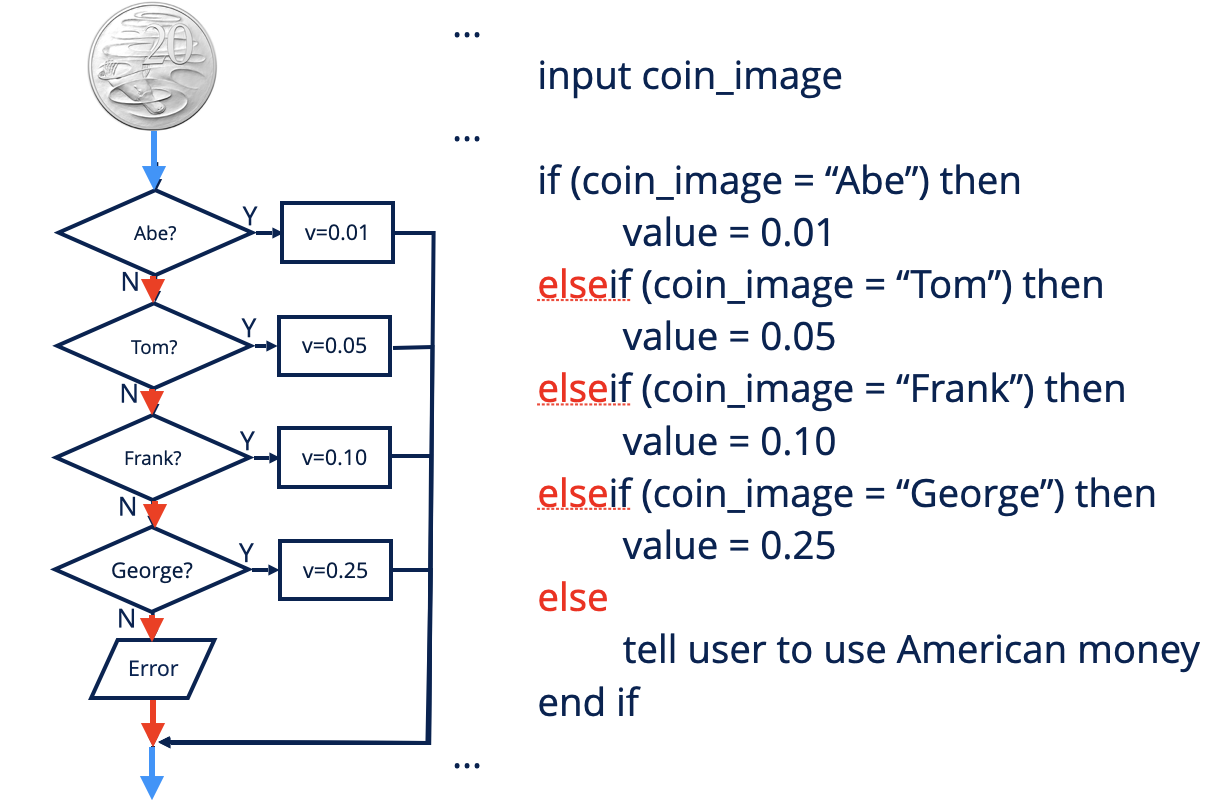
Here Else If is compressed into a single word, "elif."
#####################################################
#
# If-Elif-Else Block
#

coin = "Nickel"

print("Input Coin : ", coin)

if (coin == "Quarter"):
    value = 0.25
elif (coin == "Dime"):
    value = 0.10
elif (coin == "Nickel"):
    value = 0.05
elif (coin == "Penny"):
    value = 0.01
else:
    value = "Use the right money"

print("     value = ", value)

#
#####################################################
Input Coin :  Nickel
     value =  0.05
Single Question If Statements
This one is easy... Remember, you still have to ask the next question(s) after any of these questions.
Notice also that we can add multiple conditions.
- To add a condition, use "&" or just "and"
- To do an either-or, use "|" ("capital backslash") or just "or"
- To turn a true statement into a false one, use "not" (in other languages, it's a "!")
#####################################################
#
# Singular If Statement
#
#   (also showing multiple conditions)
#
#   remember don't be a jerk and smash things together
#     if it messes up the story telling or the readability
#     of the code!

value = 0.5

if (value >= 0.00) and (value <= 0.10):
    print(value, "is between 0.00 and 0.10")

if (value >= 0.10) & (value <= 0.50):
    print(value, "is between 0.10 and 0.50")

if (value >= 0.00) and (value <  1.00):
    print(value, "is under 1.00")

if (value <  0.50) | (value >  1.00):
    print(value, "is less than 0.50 or more than 1.00")

if ( not (value == 0) ):
    print(value, "is not equal to zero")

#
#####################################################
0.5 is between 0.10 and 0.50
0.5 is under 1.00
0.5 is not equal to zero
Activity! FizzBuzz! Because nothing promotes a student's professional development like rude noises.
Along with "Hello World," another right of passage is often the "FizzBuzz" program. This is also in your slide deck for working with loops and if-thens.
Let's recall what the pseudocode and flow chart look like!
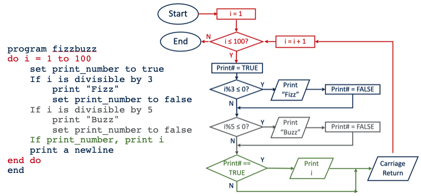
I'll repeat the pseudocode here:
program fizzbuzz
    do i = 1 to 100
        set print_number to true
        If i is divisible by 3
            print "Fizz"
            set print_number to false
        If i is divisible by 5
            print "Buzz"
            set print_number to false
        If print_number, print i
        print a newline
    end do
end
You know your duty:
#####################################################
#
# Coding FizzBuzz
#
#   Note that In the before times, printing a line,
#     backspacing and then doing a "carriage return"
#     were seperate commands.  Now they aren't but let's
#     emulate the above code the best we can!
#
#   In Python True can be written as True (capital T) or 1,
#             False can be written as False (with an big F) or 0

# <- Do Me!

for i in range(1, 100+1):
    print_number = True
    if ( (i%3) == 0):
        print("Fizz")
        print_number = False
    if ( (i%5) == 0):
        print("Buzz")
        print_number = False
    if (print_number):
        print(i)
    print("-------")

#
#####################################################
1
-------
2
-------
Fizz
-------
4
-------
Buzz
-------
Fizz
-------
7
-------
8
-------
Fizz
-------
Buzz
-------
11
-------
Fizz
-------
13
-------
14
-------
Fizz
Buzz
-------
16
-------
17
-------
Fizz
-------
19
-------
Buzz
-------
Fizz
-------
22
-------
23
-------
Fizz
-------
Buzz
-------
26
-------
Fizz
-------
28
-------
29
-------
Fizz
Buzz
-------
31
-------
32
-------
Fizz
-------
34
-------
Buzz
-------
Fizz
-------
37
-------
38
-------
Fizz
-------
Buzz
-------
41
-------
Fizz
-------
43
-------
44
-------
Fizz
Buzz
-------
46
-------
47
-------
Fizz
-------
49
-------
Buzz
-------
Fizz
-------
52
-------
53
-------
Fizz
-------
Buzz
-------
56
-------
Fizz
-------
58
-------
59
-------
Fizz
Buzz
-------
61
-------
62
-------
Fizz
-------
64
-------
Buzz
-------
Fizz
-------
67
-------
68
-------
Fizz
-------
Buzz
-------
71
-------
Fizz
-------
73
-------
74
-------
Fizz
Buzz
-------
76
-------
77
-------
Fizz
-------
79
-------
Buzz
-------
Fizz
-------
82
-------
83
-------
Fizz
-------
Buzz
-------
86
-------
Fizz
-------
88
-------
89
-------
Fizz
Buzz
-------
91
-------
92
-------
Fizz
-------
94
-------
Buzz
-------
Fizz
-------
97
-------
98
-------
Fizz
-------
Buzz
-------
Moving into Plotting
Let's get ready to do some plotting. First, we need to get some things to plot!
Let's create an independent variable representing degrees from 0 to 360 degrees.
We can also calculate some classic trig functions and plot them as simple ones.
Let's make our "x" parameter. As with other computing resources, we must turn those into Radians.
Use numpy.arange() or numpy.linspace()
#############################################
#
# Create our degrees and radians for "x"
#

# Make an array from 0 to 360 degrees (361 Values)

degrees = np.linspace(0, 360, 361) # <- Finish Me and use n=361
#
#    or
#
#   degrees = np.arange(0, 360+1)
#

# Make an array from 0 to 2 pi (361 values)

radians =   degrees * np.pi / 180. #

print("degrees = ", degrees)

print(" ")

print("radians/pi = ", radians)

#
#############################################
degrees =  [  0.   1.   2.   3.   4.   5.   6.   7.   8.   9.  10.  11.  12.  13.
  14.  15.  16.  17.  18.  19.  20.  21.  22.  23.  24.  25.  26.  27.
  28.  29.  30.  31.  32.  33.  34.  35.  36.  37.  38.  39.  40.  41.
  42.  43.  44.  45.  46.  47.  48.  49.  50.  51.  52.  53.  54.  55.
  56.  57.  58.  59.  60.  61.  62.  63.  64.  65.  66.  67.  68.  69.
  70.  71.  72.  73.  74.  75.  76.  77.  78.  79.  80.  81.  82.  83.
  84.  85.  86.  87.  88.  89.  90.  91.  92.  93.  94.  95.  96.  97.
  98.  99. 100. 101. 102. 103. 104. 105. 106. 107. 108. 109. 110. 111.
 112. 113. 114. 115. 116. 117. 118. 119. 120. 121. 122. 123. 124. 125.
 126. 127. 128. 129. 130. 131. 132. 133. 134. 135. 136. 137. 138. 139.
 140. 141. 142. 143. 144. 145. 146. 147. 148. 149. 150. 151. 152. 153.
 154. 155. 156. 157. 158. 159. 160. 161. 162. 163. 164. 165. 166. 167.
 168. 169. 170. 171. 172. 173. 174. 175. 176. 177. 178. 179. 180. 181.
 182. 183. 184. 185. 186. 187. 188. 189. 190. 191. 192. 193. 194. 195.
 196. 197. 198. 199. 200. 201. 202. 203. 204. 205. 206. 207. 208. 209.
 210. 211. 212. 213. 214. 215. 216. 217. 218. 219. 220. 221. 222. 223.
 224. 225. 226. 227. 228. 229. 230. 231. 232. 233. 234. 235. 236. 237.
 238. 239. 240. 241. 242. 243. 244. 245. 246. 247. 248. 249. 250. 251.
 252. 253. 254. 255. 256. 257. 258. 259. 260. 261. 262. 263. 264. 265.
 266. 267. 268. 269. 270. 271. 272. 273. 274. 275. 276. 277. 278. 279.
 280. 281. 282. 283. 284. 285. 286. 287. 288. 289. 290. 291. 292. 293.
 294. 295. 296. 297. 298. 299. 300. 301. 302. 303. 304. 305. 306. 307.
 308. 309. 310. 311. 312. 313. 314. 315. 316. 317. 318. 319. 320. 321.
 322. 323. 324. 325. 326. 327. 328. 329. 330. 331. 332. 333. 334. 335.
 336. 337. 338. 339. 340. 341. 342. 343. 344. 345. 346. 347. 348. 349.
 350. 351. 352. 353. 354. 355. 356. 357. 358. 359. 360.]

radians/pi =  [0.         0.01745329 0.03490659 0.05235988 0.06981317 0.08726646
 0.10471976 0.12217305 0.13962634 0.15707963 0.17453293 0.19198622
 0.20943951 0.2268928  0.2443461  0.26179939 0.27925268 0.29670597
 0.31415927 0.33161256 0.34906585 0.36651914 0.38397244 0.40142573
 0.41887902 0.43633231 0.45378561 0.4712389  0.48869219 0.50614548
 0.52359878 0.54105207 0.55850536 0.57595865 0.59341195 0.61086524
 0.62831853 0.64577182 0.66322512 0.68067841 0.6981317  0.71558499
 0.73303829 0.75049158 0.76794487 0.78539816 0.80285146 0.82030475
 0.83775804 0.85521133 0.87266463 0.89011792 0.90757121 0.9250245
 0.9424778  0.95993109 0.97738438 0.99483767 1.01229097 1.02974426
 1.04719755 1.06465084 1.08210414 1.09955743 1.11701072 1.13446401
 1.15191731 1.1693706  1.18682389 1.20427718 1.22173048 1.23918377
 1.25663706 1.27409035 1.29154365 1.30899694 1.32645023 1.34390352
 1.36135682 1.37881011 1.3962634  1.41371669 1.43116999 1.44862328
 1.46607657 1.48352986 1.50098316 1.51843645 1.53588974 1.55334303
 1.57079633 1.58824962 1.60570291 1.6231562  1.6406095  1.65806279
 1.67551608 1.69296937 1.71042267 1.72787596 1.74532925 1.76278254
 1.78023584 1.79768913 1.81514242 1.83259571 1.85004901 1.8675023
 1.88495559 1.90240888 1.91986218 1.93731547 1.95476876 1.97222205
 1.98967535 2.00712864 2.02458193 2.04203522 2.05948852 2.07694181
 2.0943951  2.11184839 2.12930169 2.14675498 2.16420827 2.18166156
 2.19911486 2.21656815 2.23402144 2.25147474 2.26892803 2.28638132
 2.30383461 2.32128791 2.3387412  2.35619449 2.37364778 2.39110108
 2.40855437 2.42600766 2.44346095 2.46091425 2.47836754 2.49582083
 2.51327412 2.53072742 2.54818071 2.565634   2.58308729 2.60054059
 2.61799388 2.63544717 2.65290046 2.67035376 2.68780705 2.70526034
 2.72271363 2.74016693 2.75762022 2.77507351 2.7925268  2.8099801
 2.82743339 2.84488668 2.86233997 2.87979327 2.89724656 2.91469985
 2.93215314 2.94960644 2.96705973 2.98451302 3.00196631 3.01941961
 3.0368729  3.05432619 3.07177948 3.08923278 3.10668607 3.12413936
 3.14159265 3.15904595 3.17649924 3.19395253 3.21140582 3.22885912
 3.24631241 3.2637657  3.28121899 3.29867229 3.31612558 3.33357887
 3.35103216 3.36848546 3.38593875 3.40339204 3.42084533 3.43829863
 3.45575192 3.47320521 3.4906585  3.5081118  3.52556509 3.54301838
 3.56047167 3.57792497 3.59537826 3.61283155 3.63028484 3.64773814
 3.66519143 3.68264472 3.70009801 3.71755131 3.7350046  3.75245789
 3.76991118 3.78736448 3.80481777 3.82227106 3.83972435 3.85717765
 3.87463094 3.89208423 3.90953752 3.92699082 3.94444411 3.9618974
 3.97935069 3.99680399 4.01425728 4.03171057 4.04916386 4.06661716
 4.08407045 4.10152374 4.11897703 4.13643033 4.15388362 4.17133691
 4.1887902  4.2062435  4.22369679 4.24115008 4.25860337 4.27605667
 4.29350996 4.31096325 4.32841654 4.34586984 4.36332313 4.38077642
 4.39822972 4.41568301 4.4331363  4.45058959 4.46804289 4.48549618
 4.50294947 4.52040276 4.53785606 4.55530935 4.57276264 4.59021593
 4.60766923 4.62512252 4.64257581 4.6600291  4.6774824  4.69493569
 4.71238898 4.72984227 4.74729557 4.76474886 4.78220215 4.79965544
 4.81710874 4.83456203 4.85201532 4.86946861 4.88692191 4.9043752
 4.92182849 4.93928178 4.95673508 4.97418837 4.99164166 5.00909495
 5.02654825 5.04400154 5.06145483 5.07890812 5.09636142 5.11381471
 5.131268   5.14872129 5.16617459 5.18362788 5.20108117 5.21853446
 5.23598776 5.25344105 5.27089434 5.28834763 5.30580093 5.32325422
 5.34070751 5.3581608  5.3756141  5.39306739 5.41052068 5.42797397
 5.44542727 5.46288056 5.48033385 5.49778714 5.51524044 5.53269373
 5.55014702 5.56760031 5.58505361 5.6025069  5.61996019 5.63741348
 5.65486678 5.67232007 5.68977336 5.70722665 5.72467995 5.74213324
 5.75958653 5.77703982 5.79449312 5.81194641 5.8293997  5.84685299
 5.86430629 5.88175958 5.89921287 5.91666616 5.93411946 5.95157275
 5.96902604 5.98647933 6.00393263 6.02138592 6.03883921 6.0562925
 6.0737458  6.09119909 6.10865238 6.12610567 6.14355897 6.16101226
 6.17846555 6.19591884 6.21337214 6.23082543 6.24827872 6.26573201
 6.28318531]
But wait a minute.
Wouldn't you think people would love converting degrees from radians?
Wouldn't you think people would love multiplying degrees by pi and then dividing by 180?
Wouldn't you think that someone would have found a better way?
If your answer was, "Sure, we ALL do!", you wouldn't be wrong.
Numpy has a function that converts degrees from radians numpy.radians() and vice versa with numpy.degrees()
#############################################
#
# Testing our handy-dandy degrees->radians function.
#

print("radians as degrees = ", np.degrees(radians))


print("degrees as radians = ", np.radians(degrees))

#
#############################################
radians as degrees =  [  0.   1.   2.   3.   4.   5.   6.   7.   8.   9.  10.  11.  12.  13.
  14.  15.  16.  17.  18.  19.  20.  21.  22.  23.  24.  25.  26.  27.
  28.  29.  30.  31.  32.  33.  34.  35.  36.  37.  38.  39.  40.  41.
  42.  43.  44.  45.  46.  47.  48.  49.  50.  51.  52.  53.  54.  55.
  56.  57.  58.  59.  60.  61.  62.  63.  64.  65.  66.  67.  68.  69.
  70.  71.  72.  73.  74.  75.  76.  77.  78.  79.  80.  81.  82.  83.
  84.  85.  86.  87.  88.  89.  90.  91.  92.  93.  94.  95.  96.  97.
  98.  99. 100. 101. 102. 103. 104. 105. 106. 107. 108. 109. 110. 111.
 112. 113. 114. 115. 116. 117. 118. 119. 120. 121. 122. 123. 124. 125.
 126. 127. 128. 129. 130. 131. 132. 133. 134. 135. 136. 137. 138. 139.
 140. 141. 142. 143. 144. 145. 146. 147. 148. 149. 150. 151. 152. 153.
 154. 155. 156. 157. 158. 159. 160. 161. 162. 163. 164. 165. 166. 167.
 168. 169. 170. 171. 172. 173. 174. 175. 176. 177. 178. 179. 180. 181.
 182. 183. 184. 185. 186. 187. 188. 189. 190. 191. 192. 193. 194. 195.
 196. 197. 198. 199. 200. 201. 202. 203. 204. 205. 206. 207. 208. 209.
 210. 211. 212. 213. 214. 215. 216. 217. 218. 219. 220. 221. 222. 223.
 224. 225. 226. 227. 228. 229. 230. 231. 232. 233. 234. 235. 236. 237.
 238. 239. 240. 241. 242. 243. 244. 245. 246. 247. 248. 249. 250. 251.
 252. 253. 254. 255. 256. 257. 258. 259. 260. 261. 262. 263. 264. 265.
 266. 267. 268. 269. 270. 271. 272. 273. 274. 275. 276. 277. 278. 279.
 280. 281. 282. 283. 284. 285. 286. 287. 288. 289. 290. 291. 292. 293.
 294. 295. 296. 297. 298. 299. 300. 301. 302. 303. 304. 305. 306. 307.
 308. 309. 310. 311. 312. 313. 314. 315. 316. 317. 318. 319. 320. 321.
 322. 323. 324. 325. 326. 327. 328. 329. 330. 331. 332. 333. 334. 335.
 336. 337. 338. 339. 340. 341. 342. 343. 344. 345. 346. 347. 348. 349.
 350. 351. 352. 353. 354. 355. 356. 357. 358. 359. 360.]
degrees as radians =  [0.         0.01745329 0.03490659 0.05235988 0.06981317 0.08726646
 0.10471976 0.12217305 0.13962634 0.15707963 0.17453293 0.19198622
 0.20943951 0.2268928  0.2443461  0.26179939 0.27925268 0.29670597
 0.31415927 0.33161256 0.34906585 0.36651914 0.38397244 0.40142573
 0.41887902 0.43633231 0.45378561 0.4712389  0.48869219 0.50614548
 0.52359878 0.54105207 0.55850536 0.57595865 0.59341195 0.61086524
 0.62831853 0.64577182 0.66322512 0.68067841 0.6981317  0.71558499
 0.73303829 0.75049158 0.76794487 0.78539816 0.80285146 0.82030475
 0.83775804 0.85521133 0.87266463 0.89011792 0.90757121 0.9250245
 0.9424778  0.95993109 0.97738438 0.99483767 1.01229097 1.02974426
 1.04719755 1.06465084 1.08210414 1.09955743 1.11701072 1.13446401
 1.15191731 1.1693706  1.18682389 1.20427718 1.22173048 1.23918377
 1.25663706 1.27409035 1.29154365 1.30899694 1.32645023 1.34390352
 1.36135682 1.37881011 1.3962634  1.41371669 1.43116999 1.44862328
 1.46607657 1.48352986 1.50098316 1.51843645 1.53588974 1.55334303
 1.57079633 1.58824962 1.60570291 1.6231562  1.6406095  1.65806279
 1.67551608 1.69296937 1.71042267 1.72787596 1.74532925 1.76278254
 1.78023584 1.79768913 1.81514242 1.83259571 1.85004901 1.8675023
 1.88495559 1.90240888 1.91986218 1.93731547 1.95476876 1.97222205
 1.98967535 2.00712864 2.02458193 2.04203522 2.05948852 2.07694181
 2.0943951  2.11184839 2.12930169 2.14675498 2.16420827 2.18166156
 2.19911486 2.21656815 2.23402144 2.25147474 2.26892803 2.28638132
 2.30383461 2.32128791 2.3387412  2.35619449 2.37364778 2.39110108
 2.40855437 2.42600766 2.44346095 2.46091425 2.47836754 2.49582083
 2.51327412 2.53072742 2.54818071 2.565634   2.58308729 2.60054059
 2.61799388 2.63544717 2.65290046 2.67035376 2.68780705 2.70526034
 2.72271363 2.74016693 2.75762022 2.77507351 2.7925268  2.8099801
 2.82743339 2.84488668 2.86233997 2.87979327 2.89724656 2.91469985
 2.93215314 2.94960644 2.96705973 2.98451302 3.00196631 3.01941961
 3.0368729  3.05432619 3.07177948 3.08923278 3.10668607 3.12413936
 3.14159265 3.15904595 3.17649924 3.19395253 3.21140582 3.22885912
 3.24631241 3.2637657  3.28121899 3.29867229 3.31612558 3.33357887
 3.35103216 3.36848546 3.38593875 3.40339204 3.42084533 3.43829863
 3.45575192 3.47320521 3.4906585  3.5081118  3.52556509 3.54301838
 3.56047167 3.57792497 3.59537826 3.61283155 3.63028484 3.64773814
 3.66519143 3.68264472 3.70009801 3.71755131 3.7350046  3.75245789
 3.76991118 3.78736448 3.80481777 3.82227106 3.83972435 3.85717765
 3.87463094 3.89208423 3.90953752 3.92699082 3.94444411 3.9618974
 3.97935069 3.99680399 4.01425728 4.03171057 4.04916386 4.06661716
 4.08407045 4.10152374 4.11897703 4.13643033 4.15388362 4.17133691
 4.1887902  4.2062435  4.22369679 4.24115008 4.25860337 4.27605667
 4.29350996 4.31096325 4.32841654 4.34586984 4.36332313 4.38077642
 4.39822972 4.41568301 4.4331363  4.45058959 4.46804289 4.48549618
 4.50294947 4.52040276 4.53785606 4.55530935 4.57276264 4.59021593
 4.60766923 4.62512252 4.64257581 4.6600291  4.6774824  4.69493569
 4.71238898 4.72984227 4.74729557 4.76474886 4.78220215 4.79965544
 4.81710874 4.83456203 4.85201532 4.86946861 4.88692191 4.9043752
 4.92182849 4.93928178 4.95673508 4.97418837 4.99164166 5.00909495
 5.02654825 5.04400154 5.06145483 5.07890812 5.09636142 5.11381471
 5.131268   5.14872129 5.16617459 5.18362788 5.20108117 5.21853446
 5.23598776 5.25344105 5.27089434 5.28834763 5.30580093 5.32325422
 5.34070751 5.3581608  5.3756141  5.39306739 5.41052068 5.42797397
 5.44542727 5.46288056 5.48033385 5.49778714 5.51524044 5.53269373
 5.55014702 5.56760031 5.58505361 5.6025069  5.61996019 5.63741348
 5.65486678 5.67232007 5.68977336 5.70722665 5.72467995 5.74213324
 5.75958653 5.77703982 5.79449312 5.81194641 5.8293997  5.84685299
 5.86430629 5.88175958 5.89921287 5.91666616 5.93411946 5.95157275
 5.96902604 5.98647933 6.00393263 6.02138592 6.03883921 6.0562925
 6.0737458  6.09119909 6.10865238 6.12610567 6.14355897 6.16101226
 6.17846555 6.19591884 6.21337214 6.23082543 6.24827872 6.26573201
 6.28318531]
Create our trig functions...
We're going to use some basic trig functions: numpy.sin(), numpy.cos(), and numpy.tan().
The good news is that this type of math function does not require you to have 361 individual calls to the functions.
That is because these are "universal functions," or "ufuncs" in Python. Even though there is one output value, you can send a series or array of values into it to output a return vector. The nerd term for this is "vectorization."
We will need to revisit this term next week. But for now, we will take advantage of it.
#############################################
#
# Applying our trig functions to our radians array
#

cos_array = np.cos(radians)

sin_array = np.sin(radians)

tan_array = np.tan(radians)

print("cos_array = ", cos_array)

print("")

print("sin_array = ", sin_array)

print("")

print("tan_array = ", tan_array)

#
#############################################
cos_array =  [ 1.00000000e+00  9.99847695e-01  9.99390827e-01  9.98629535e-01
  9.97564050e-01  9.96194698e-01  9.94521895e-01  9.92546152e-01
  9.90268069e-01  9.87688341e-01  9.84807753e-01  9.81627183e-01
  9.78147601e-01  9.74370065e-01  9.70295726e-01  9.65925826e-01
  9.61261696e-01  9.56304756e-01  9.51056516e-01  9.45518576e-01
  9.39692621e-01  9.33580426e-01  9.27183855e-01  9.20504853e-01
  9.13545458e-01  9.06307787e-01  8.98794046e-01  8.91006524e-01
  8.82947593e-01  8.74619707e-01  8.66025404e-01  8.57167301e-01
  8.48048096e-01  8.38670568e-01  8.29037573e-01  8.19152044e-01
  8.09016994e-01  7.98635510e-01  7.88010754e-01  7.77145961e-01
  7.66044443e-01  7.54709580e-01  7.43144825e-01  7.31353702e-01
  7.19339800e-01  7.07106781e-01  6.94658370e-01  6.81998360e-01
  6.69130606e-01  6.56059029e-01  6.42787610e-01  6.29320391e-01
  6.15661475e-01  6.01815023e-01  5.87785252e-01  5.73576436e-01
  5.59192903e-01  5.44639035e-01  5.29919264e-01  5.15038075e-01
  5.00000000e-01  4.84809620e-01  4.69471563e-01  4.53990500e-01
  4.38371147e-01  4.22618262e-01  4.06736643e-01  3.90731128e-01
  3.74606593e-01  3.58367950e-01  3.42020143e-01  3.25568154e-01
  3.09016994e-01  2.92371705e-01  2.75637356e-01  2.58819045e-01
  2.41921896e-01  2.24951054e-01  2.07911691e-01  1.90808995e-01
  1.73648178e-01  1.56434465e-01  1.39173101e-01  1.21869343e-01
  1.04528463e-01  8.71557427e-02  6.97564737e-02  5.23359562e-02
  3.48994967e-02  1.74524064e-02  6.12323400e-17 -1.74524064e-02
 -3.48994967e-02 -5.23359562e-02 -6.97564737e-02 -8.71557427e-02
 -1.04528463e-01 -1.21869343e-01 -1.39173101e-01 -1.56434465e-01
 -1.73648178e-01 -1.90808995e-01 -2.07911691e-01 -2.24951054e-01
 -2.41921896e-01 -2.58819045e-01 -2.75637356e-01 -2.92371705e-01
 -3.09016994e-01 -3.25568154e-01 -3.42020143e-01 -3.58367950e-01
 -3.74606593e-01 -3.90731128e-01 -4.06736643e-01 -4.22618262e-01
 -4.38371147e-01 -4.53990500e-01 -4.69471563e-01 -4.84809620e-01
 -5.00000000e-01 -5.15038075e-01 -5.29919264e-01 -5.44639035e-01
 -5.59192903e-01 -5.73576436e-01 -5.87785252e-01 -6.01815023e-01
 -6.15661475e-01 -6.29320391e-01 -6.42787610e-01 -6.56059029e-01
 -6.69130606e-01 -6.81998360e-01 -6.94658370e-01 -7.07106781e-01
 -7.19339800e-01 -7.31353702e-01 -7.43144825e-01 -7.54709580e-01
 -7.66044443e-01 -7.77145961e-01 -7.88010754e-01 -7.98635510e-01
 -8.09016994e-01 -8.19152044e-01 -8.29037573e-01 -8.38670568e-01
 -8.48048096e-01 -8.57167301e-01 -8.66025404e-01 -8.74619707e-01
 -8.82947593e-01 -8.91006524e-01 -8.98794046e-01 -9.06307787e-01
 -9.13545458e-01 -9.20504853e-01 -9.27183855e-01 -9.33580426e-01
 -9.39692621e-01 -9.45518576e-01 -9.51056516e-01 -9.56304756e-01
 -9.61261696e-01 -9.65925826e-01 -9.70295726e-01 -9.74370065e-01
 -9.78147601e-01 -9.81627183e-01 -9.84807753e-01 -9.87688341e-01
 -9.90268069e-01 -9.92546152e-01 -9.94521895e-01 -9.96194698e-01
 -9.97564050e-01 -9.98629535e-01 -9.99390827e-01 -9.99847695e-01
 -1.00000000e+00 -9.99847695e-01 -9.99390827e-01 -9.98629535e-01
 -9.97564050e-01 -9.96194698e-01 -9.94521895e-01 -9.92546152e-01
 -9.90268069e-01 -9.87688341e-01 -9.84807753e-01 -9.81627183e-01
 -9.78147601e-01 -9.74370065e-01 -9.70295726e-01 -9.65925826e-01
 -9.61261696e-01 -9.56304756e-01 -9.51056516e-01 -9.45518576e-01
 -9.39692621e-01 -9.33580426e-01 -9.27183855e-01 -9.20504853e-01
 -9.13545458e-01 -9.06307787e-01 -8.98794046e-01 -8.91006524e-01
 -8.82947593e-01 -8.74619707e-01 -8.66025404e-01 -8.57167301e-01
 -8.48048096e-01 -8.38670568e-01 -8.29037573e-01 -8.19152044e-01
 -8.09016994e-01 -7.98635510e-01 -7.88010754e-01 -7.77145961e-01
 -7.66044443e-01 -7.54709580e-01 -7.43144825e-01 -7.31353702e-01
 -7.19339800e-01 -7.07106781e-01 -6.94658370e-01 -6.81998360e-01
 -6.69130606e-01 -6.56059029e-01 -6.42787610e-01 -6.29320391e-01
 -6.15661475e-01 -6.01815023e-01 -5.87785252e-01 -5.73576436e-01
 -5.59192903e-01 -5.44639035e-01 -5.29919264e-01 -5.15038075e-01
 -5.00000000e-01 -4.84809620e-01 -4.69471563e-01 -4.53990500e-01
 -4.38371147e-01 -4.22618262e-01 -4.06736643e-01 -3.90731128e-01
 -3.74606593e-01 -3.58367950e-01 -3.42020143e-01 -3.25568154e-01
 -3.09016994e-01 -2.92371705e-01 -2.75637356e-01 -2.58819045e-01
 -2.41921896e-01 -2.24951054e-01 -2.07911691e-01 -1.90808995e-01
 -1.73648178e-01 -1.56434465e-01 -1.39173101e-01 -1.21869343e-01
 -1.04528463e-01 -8.71557427e-02 -6.97564737e-02 -5.23359562e-02
 -3.48994967e-02 -1.74524064e-02 -1.83697020e-16  1.74524064e-02
  3.48994967e-02  5.23359562e-02  6.97564737e-02  8.71557427e-02
  1.04528463e-01  1.21869343e-01  1.39173101e-01  1.56434465e-01
  1.73648178e-01  1.90808995e-01  2.07911691e-01  2.24951054e-01
  2.41921896e-01  2.58819045e-01  2.75637356e-01  2.92371705e-01
  3.09016994e-01  3.25568154e-01  3.42020143e-01  3.58367950e-01
  3.74606593e-01  3.90731128e-01  4.06736643e-01  4.22618262e-01
  4.38371147e-01  4.53990500e-01  4.69471563e-01  4.84809620e-01
  5.00000000e-01  5.15038075e-01  5.29919264e-01  5.44639035e-01
  5.59192903e-01  5.73576436e-01  5.87785252e-01  6.01815023e-01
  6.15661475e-01  6.29320391e-01  6.42787610e-01  6.56059029e-01
  6.69130606e-01  6.81998360e-01  6.94658370e-01  7.07106781e-01
  7.19339800e-01  7.31353702e-01  7.43144825e-01  7.54709580e-01
  7.66044443e-01  7.77145961e-01  7.88010754e-01  7.98635510e-01
  8.09016994e-01  8.19152044e-01  8.29037573e-01  8.38670568e-01
  8.48048096e-01  8.57167301e-01  8.66025404e-01  8.74619707e-01
  8.82947593e-01  8.91006524e-01  8.98794046e-01  9.06307787e-01
  9.13545458e-01  9.20504853e-01  9.27183855e-01  9.33580426e-01
  9.39692621e-01  9.45518576e-01  9.51056516e-01  9.56304756e-01
  9.61261696e-01  9.65925826e-01  9.70295726e-01  9.74370065e-01
  9.78147601e-01  9.81627183e-01  9.84807753e-01  9.87688341e-01
  9.90268069e-01  9.92546152e-01  9.94521895e-01  9.96194698e-01
  9.97564050e-01  9.98629535e-01  9.99390827e-01  9.99847695e-01
  1.00000000e+00]

sin_array =  [ 0.00000000e+00  1.74524064e-02  3.48994967e-02  5.23359562e-02
  6.97564737e-02  8.71557427e-02  1.04528463e-01  1.21869343e-01
  1.39173101e-01  1.56434465e-01  1.73648178e-01  1.90808995e-01
  2.07911691e-01  2.24951054e-01  2.41921896e-01  2.58819045e-01
  2.75637356e-01  2.92371705e-01  3.09016994e-01  3.25568154e-01
  3.42020143e-01  3.58367950e-01  3.74606593e-01  3.90731128e-01
  4.06736643e-01  4.22618262e-01  4.38371147e-01  4.53990500e-01
  4.69471563e-01  4.84809620e-01  5.00000000e-01  5.15038075e-01
  5.29919264e-01  5.44639035e-01  5.59192903e-01  5.73576436e-01
  5.87785252e-01  6.01815023e-01  6.15661475e-01  6.29320391e-01
  6.42787610e-01  6.56059029e-01  6.69130606e-01  6.81998360e-01
  6.94658370e-01  7.07106781e-01  7.19339800e-01  7.31353702e-01
  7.43144825e-01  7.54709580e-01  7.66044443e-01  7.77145961e-01
  7.88010754e-01  7.98635510e-01  8.09016994e-01  8.19152044e-01
  8.29037573e-01  8.38670568e-01  8.48048096e-01  8.57167301e-01
  8.66025404e-01  8.74619707e-01  8.82947593e-01  8.91006524e-01
  8.98794046e-01  9.06307787e-01  9.13545458e-01  9.20504853e-01
  9.27183855e-01  9.33580426e-01  9.39692621e-01  9.45518576e-01
  9.51056516e-01  9.56304756e-01  9.61261696e-01  9.65925826e-01
  9.70295726e-01  9.74370065e-01  9.78147601e-01  9.81627183e-01
  9.84807753e-01  9.87688341e-01  9.90268069e-01  9.92546152e-01
  9.94521895e-01  9.96194698e-01  9.97564050e-01  9.98629535e-01
  9.99390827e-01  9.99847695e-01  1.00000000e+00  9.99847695e-01
  9.99390827e-01  9.98629535e-01  9.97564050e-01  9.96194698e-01
  9.94521895e-01  9.92546152e-01  9.90268069e-01  9.87688341e-01
  9.84807753e-01  9.81627183e-01  9.78147601e-01  9.74370065e-01
  9.70295726e-01  9.65925826e-01  9.61261696e-01  9.56304756e-01
  9.51056516e-01  9.45518576e-01  9.39692621e-01  9.33580426e-01
  9.27183855e-01  9.20504853e-01  9.13545458e-01  9.06307787e-01
  8.98794046e-01  8.91006524e-01  8.82947593e-01  8.74619707e-01
  8.66025404e-01  8.57167301e-01  8.48048096e-01  8.38670568e-01
  8.29037573e-01  8.19152044e-01  8.09016994e-01  7.98635510e-01
  7.88010754e-01  7.77145961e-01  7.66044443e-01  7.54709580e-01
  7.43144825e-01  7.31353702e-01  7.19339800e-01  7.07106781e-01
  6.94658370e-01  6.81998360e-01  6.69130606e-01  6.56059029e-01
  6.42787610e-01  6.29320391e-01  6.15661475e-01  6.01815023e-01
  5.87785252e-01  5.73576436e-01  5.59192903e-01  5.44639035e-01
  5.29919264e-01  5.15038075e-01  5.00000000e-01  4.84809620e-01
  4.69471563e-01  4.53990500e-01  4.38371147e-01  4.22618262e-01
  4.06736643e-01  3.90731128e-01  3.74606593e-01  3.58367950e-01
  3.42020143e-01  3.25568154e-01  3.09016994e-01  2.92371705e-01
  2.75637356e-01  2.58819045e-01  2.41921896e-01  2.24951054e-01
  2.07911691e-01  1.90808995e-01  1.73648178e-01  1.56434465e-01
  1.39173101e-01  1.21869343e-01  1.04528463e-01  8.71557427e-02
  6.97564737e-02  5.23359562e-02  3.48994967e-02  1.74524064e-02
  1.22464680e-16 -1.74524064e-02 -3.48994967e-02 -5.23359562e-02
 -6.97564737e-02 -8.71557427e-02 -1.04528463e-01 -1.21869343e-01
 -1.39173101e-01 -1.56434465e-01 -1.73648178e-01 -1.90808995e-01
 -2.07911691e-01 -2.24951054e-01 -2.41921896e-01 -2.58819045e-01
 -2.75637356e-01 -2.92371705e-01 -3.09016994e-01 -3.25568154e-01
 -3.42020143e-01 -3.58367950e-01 -3.74606593e-01 -3.90731128e-01
 -4.06736643e-01 -4.22618262e-01 -4.38371147e-01 -4.53990500e-01
 -4.69471563e-01 -4.84809620e-01 -5.00000000e-01 -5.15038075e-01
 -5.29919264e-01 -5.44639035e-01 -5.59192903e-01 -5.73576436e-01
 -5.87785252e-01 -6.01815023e-01 -6.15661475e-01 -6.29320391e-01
 -6.42787610e-01 -6.56059029e-01 -6.69130606e-01 -6.81998360e-01
 -6.94658370e-01 -7.07106781e-01 -7.19339800e-01 -7.31353702e-01
 -7.43144825e-01 -7.54709580e-01 -7.66044443e-01 -7.77145961e-01
 -7.88010754e-01 -7.98635510e-01 -8.09016994e-01 -8.19152044e-01
 -8.29037573e-01 -8.38670568e-01 -8.48048096e-01 -8.57167301e-01
 -8.66025404e-01 -8.74619707e-01 -8.82947593e-01 -8.91006524e-01
 -8.98794046e-01 -9.06307787e-01 -9.13545458e-01 -9.20504853e-01
 -9.27183855e-01 -9.33580426e-01 -9.39692621e-01 -9.45518576e-01
 -9.51056516e-01 -9.56304756e-01 -9.61261696e-01 -9.65925826e-01
 -9.70295726e-01 -9.74370065e-01 -9.78147601e-01 -9.81627183e-01
 -9.84807753e-01 -9.87688341e-01 -9.90268069e-01 -9.92546152e-01
 -9.94521895e-01 -9.96194698e-01 -9.97564050e-01 -9.98629535e-01
 -9.99390827e-01 -9.99847695e-01 -1.00000000e+00 -9.99847695e-01
 -9.99390827e-01 -9.98629535e-01 -9.97564050e-01 -9.96194698e-01
 -9.94521895e-01 -9.92546152e-01 -9.90268069e-01 -9.87688341e-01
 -9.84807753e-01 -9.81627183e-01 -9.78147601e-01 -9.74370065e-01
 -9.70295726e-01 -9.65925826e-01 -9.61261696e-01 -9.56304756e-01
 -9.51056516e-01 -9.45518576e-01 -9.39692621e-01 -9.33580426e-01
 -9.27183855e-01 -9.20504853e-01 -9.13545458e-01 -9.06307787e-01
 -8.98794046e-01 -8.91006524e-01 -8.82947593e-01 -8.74619707e-01
 -8.66025404e-01 -8.57167301e-01 -8.48048096e-01 -8.38670568e-01
 -8.29037573e-01 -8.19152044e-01 -8.09016994e-01 -7.98635510e-01
 -7.88010754e-01 -7.77145961e-01 -7.66044443e-01 -7.54709580e-01
 -7.43144825e-01 -7.31353702e-01 -7.19339800e-01 -7.07106781e-01
 -6.94658370e-01 -6.81998360e-01 -6.69130606e-01 -6.56059029e-01
 -6.42787610e-01 -6.29320391e-01 -6.15661475e-01 -6.01815023e-01
 -5.87785252e-01 -5.73576436e-01 -5.59192903e-01 -5.44639035e-01
 -5.29919264e-01 -5.15038075e-01 -5.00000000e-01 -4.84809620e-01
 -4.69471563e-01 -4.53990500e-01 -4.38371147e-01 -4.22618262e-01
 -4.06736643e-01 -3.90731128e-01 -3.74606593e-01 -3.58367950e-01
 -3.42020143e-01 -3.25568154e-01 -3.09016994e-01 -2.92371705e-01
 -2.75637356e-01 -2.58819045e-01 -2.41921896e-01 -2.24951054e-01
 -2.07911691e-01 -1.90808995e-01 -1.73648178e-01 -1.56434465e-01
 -1.39173101e-01 -1.21869343e-01 -1.04528463e-01 -8.71557427e-02
 -6.97564737e-02 -5.23359562e-02 -3.48994967e-02 -1.74524064e-02
 -2.44929360e-16]

tan_array =  [ 0.00000000e+00  1.74550649e-02  3.49207695e-02  5.24077793e-02
  6.99268119e-02  8.74886635e-02  1.05104235e-01  1.22784561e-01
  1.40540835e-01  1.58384440e-01  1.76326981e-01  1.94380309e-01
  2.12556562e-01  2.30868191e-01  2.49328003e-01  2.67949192e-01
  2.86745386e-01  3.05730681e-01  3.24919696e-01  3.44327613e-01
  3.63970234e-01  3.83864035e-01  4.04026226e-01  4.24474816e-01
  4.45228685e-01  4.66307658e-01  4.87732589e-01  5.09525449e-01
  5.31709432e-01  5.54309051e-01  5.77350269e-01  6.00860619e-01
  6.24869352e-01  6.49407593e-01  6.74508517e-01  7.00207538e-01
  7.26542528e-01  7.53554050e-01  7.81285627e-01  8.09784033e-01
  8.39099631e-01  8.69286738e-01  9.00404044e-01  9.32515086e-01
  9.65688775e-01  1.00000000e+00  1.03553031e+00  1.07236871e+00
  1.11061251e+00  1.15036841e+00  1.19175359e+00  1.23489716e+00
  1.27994163e+00  1.32704482e+00  1.37638192e+00  1.42814801e+00
  1.48256097e+00  1.53986496e+00  1.60033453e+00  1.66427948e+00
  1.73205081e+00  1.80404776e+00  1.88072647e+00  1.96261051e+00
  2.05030384e+00  2.14450692e+00  2.24603677e+00  2.35585237e+00
  2.47508685e+00  2.60508906e+00  2.74747742e+00  2.90421088e+00
  3.07768354e+00  3.27085262e+00  3.48741444e+00  3.73205081e+00
  4.01078093e+00  4.33147587e+00  4.70463011e+00  5.14455402e+00
  5.67128182e+00  6.31375151e+00  7.11536972e+00  8.14434643e+00
  9.51436445e+00  1.14300523e+01  1.43006663e+01  1.90811367e+01
  2.86362533e+01  5.72899616e+01  1.63312394e+16 -5.72899616e+01
 -2.86362533e+01 -1.90811367e+01 -1.43006663e+01 -1.14300523e+01
 -9.51436445e+00 -8.14434643e+00 -7.11536972e+00 -6.31375151e+00
 -5.67128182e+00 -5.14455402e+00 -4.70463011e+00 -4.33147587e+00
 -4.01078093e+00 -3.73205081e+00 -3.48741444e+00 -3.27085262e+00
 -3.07768354e+00 -2.90421088e+00 -2.74747742e+00 -2.60508906e+00
 -2.47508685e+00 -2.35585237e+00 -2.24603677e+00 -2.14450692e+00
 -2.05030384e+00 -1.96261051e+00 -1.88072647e+00 -1.80404776e+00
 -1.73205081e+00 -1.66427948e+00 -1.60033453e+00 -1.53986496e+00
 -1.48256097e+00 -1.42814801e+00 -1.37638192e+00 -1.32704482e+00
 -1.27994163e+00 -1.23489716e+00 -1.19175359e+00 -1.15036841e+00
 -1.11061251e+00 -1.07236871e+00 -1.03553031e+00 -1.00000000e+00
 -9.65688775e-01 -9.32515086e-01 -9.00404044e-01 -8.69286738e-01
 -8.39099631e-01 -8.09784033e-01 -7.81285627e-01 -7.53554050e-01
 -7.26542528e-01 -7.00207538e-01 -6.74508517e-01 -6.49407593e-01
 -6.24869352e-01 -6.00860619e-01 -5.77350269e-01 -5.54309051e-01
 -5.31709432e-01 -5.09525449e-01 -4.87732589e-01 -4.66307658e-01
 -4.45228685e-01 -4.24474816e-01 -4.04026226e-01 -3.83864035e-01
 -3.63970234e-01 -3.44327613e-01 -3.24919696e-01 -3.05730681e-01
 -2.86745386e-01 -2.67949192e-01 -2.49328003e-01 -2.30868191e-01
 -2.12556562e-01 -1.94380309e-01 -1.76326981e-01 -1.58384440e-01
 -1.40540835e-01 -1.22784561e-01 -1.05104235e-01 -8.74886635e-02
 -6.99268119e-02 -5.24077793e-02 -3.49207695e-02 -1.74550649e-02
 -1.22464680e-16  1.74550649e-02  3.49207695e-02  5.24077793e-02
  6.99268119e-02  8.74886635e-02  1.05104235e-01  1.22784561e-01
  1.40540835e-01  1.58384440e-01  1.76326981e-01  1.94380309e-01
  2.12556562e-01  2.30868191e-01  2.49328003e-01  2.67949192e-01
  2.86745386e-01  3.05730681e-01  3.24919696e-01  3.44327613e-01
  3.63970234e-01  3.83864035e-01  4.04026226e-01  4.24474816e-01
  4.45228685e-01  4.66307658e-01  4.87732589e-01  5.09525449e-01
  5.31709432e-01  5.54309051e-01  5.77350269e-01  6.00860619e-01
  6.24869352e-01  6.49407593e-01  6.74508517e-01  7.00207538e-01
  7.26542528e-01  7.53554050e-01  7.81285627e-01  8.09784033e-01
  8.39099631e-01  8.69286738e-01  9.00404044e-01  9.32515086e-01
  9.65688775e-01  1.00000000e+00  1.03553031e+00  1.07236871e+00
  1.11061251e+00  1.15036841e+00  1.19175359e+00  1.23489716e+00
  1.27994163e+00  1.32704482e+00  1.37638192e+00  1.42814801e+00
  1.48256097e+00  1.53986496e+00  1.60033453e+00  1.66427948e+00
  1.73205081e+00  1.80404776e+00  1.88072647e+00  1.96261051e+00
  2.05030384e+00  2.14450692e+00  2.24603677e+00  2.35585237e+00
  2.47508685e+00  2.60508906e+00  2.74747742e+00  2.90421088e+00
  3.07768354e+00  3.27085262e+00  3.48741444e+00  3.73205081e+00
  4.01078093e+00  4.33147587e+00  4.70463011e+00  5.14455402e+00
  5.67128182e+00  6.31375151e+00  7.11536972e+00  8.14434643e+00
  9.51436445e+00  1.14300523e+01  1.43006663e+01  1.90811367e+01
  2.86362533e+01  5.72899616e+01  5.44374645e+15 -5.72899616e+01
 -2.86362533e+01 -1.90811367e+01 -1.43006663e+01 -1.14300523e+01
 -9.51436445e+00 -8.14434643e+00 -7.11536972e+00 -6.31375151e+00
 -5.67128182e+00 -5.14455402e+00 -4.70463011e+00 -4.33147587e+00
 -4.01078093e+00 -3.73205081e+00 -3.48741444e+00 -3.27085262e+00
 -3.07768354e+00 -2.90421088e+00 -2.74747742e+00 -2.60508906e+00
 -2.47508685e+00 -2.35585237e+00 -2.24603677e+00 -2.14450692e+00
 -2.05030384e+00 -1.96261051e+00 -1.88072647e+00 -1.80404776e+00
 -1.73205081e+00 -1.66427948e+00 -1.60033453e+00 -1.53986496e+00
 -1.48256097e+00 -1.42814801e+00 -1.37638192e+00 -1.32704482e+00
 -1.27994163e+00 -1.23489716e+00 -1.19175359e+00 -1.15036841e+00
 -1.11061251e+00 -1.07236871e+00 -1.03553031e+00 -1.00000000e+00
 -9.65688775e-01 -9.32515086e-01 -9.00404044e-01 -8.69286738e-01
 -8.39099631e-01 -8.09784033e-01 -7.81285627e-01 -7.53554050e-01
 -7.26542528e-01 -7.00207538e-01 -6.74508517e-01 -6.49407593e-01
 -6.24869352e-01 -6.00860619e-01 -5.77350269e-01 -5.54309051e-01
 -5.31709432e-01 -5.09525449e-01 -4.87732589e-01 -4.66307658e-01
 -4.45228685e-01 -4.24474816e-01 -4.04026226e-01 -3.83864035e-01
 -3.63970234e-01 -3.44327613e-01 -3.24919696e-01 -3.05730681e-01
 -2.86745386e-01 -2.67949192e-01 -2.49328003e-01 -2.30868191e-01
 -2.12556562e-01 -1.94380309e-01 -1.76326981e-01 -1.58384440e-01
 -1.40540835e-01 -1.22784561e-01 -1.05104235e-01 -8.74886635e-02
 -6.99268119e-02 -5.24077793e-02 -3.49207695e-02 -1.74550649e-02
 -2.44929360e-16]
Plotting with Matplotlib.
Well those printed array of numbers are all-and-good, but honestly, nothing conveys the meeting of these functions like a graph.
This brings is to the matplotlib environment. Most plotting tools leverage matplotlib including highly specialized graphs and mapping libraries.
If you've worked with MATLAB before, some of this is going to be eerily familiar. The syntax here will be very similar to MATLAB right down to customizing the symbols on a series.
If you haven't worked with MATLAB, we will do a simple demo of an x-y plot here in short increments.
Warning, there is an easy way to plot in Python, and the way all the online examples tell you how to plot in Python...
Before we move forward a few points about working with graphs in python.
There are ways to make plots that for the most part maintain my prefered adage of "maximum satisfaction with minimal effort" (stolen from TV cooking presenter Nigella Lawson).
However to make really fancy ones featured in the galleries that accompany the online help for matplotlib and seaborn, you need to use some of the more advanced features that often become very confusing.
This for me was another "rage-quit" point when I did my pivot to Python from my past tools. I'll be handing you a tutorial on how to get fancy with (hopefully) minimal screams and profanity later in the course.
The good news is that, for this class, we mostly won't be using the more advanved elements of plotting.
The plot Command
Simple x-y plots have one or two array arguments.
If it's just one argument, it plots the data along the y axis and the x-axis is just the number of the observation.
If it's two arguments, then it's plotting a traditional x-y plot.
Beyond that there are a suite of modifiers to manage the color, symbol, linestyle, etc.
Unless you use it daily, you're probably not going to have instant recall of most of them.
No problem: The manual page for matlibplot.pyplot.plot() has details.
Let's start by ploting a very simple plot of our above case., starting with the defaults, then getting progressively fancier by gradually adding "bell-and-whistle" functions that can be found here.
To move forward here, I am going to be doing a lot of repetative plotting, gradually adding "features." (This is because one of my peeves if you look at some of the example galleries on how to plot in python, they drop EVERYTHING into a single script, often with little explaination with the plots go. File that under yet another thing that will get me to rage-quit when adopting a new work environment.)
So let's start with a very simple x-y plot.
#############################################
#
# Default X-Y plot
#

# <- Do Me and Plot Degrees vs Sine

plt.plot(degrees, sin_array)

#
#############################################
[<matplotlib.lines.Line2D at 0x1073b07d0>]

Note that above the plot what looks like a label for the top of the graph. It's not a label. Rather it is a report on the object ID. It's not needed for the consumer of the plot. One way to get rid of it is to add the command plt.show() when you are ready to display the plot. This also lets you display more than on plot in a single code block in the Jupyter environment so I recommend that you use it as a best practice.
For example:
#############################################
#
# Default X-Y plots with the plt.show option.
#


print("This isn't a label but the graph below is a sine plot")

# <- Do Me and Plot Degrees vs Sine

plt.plot(degrees, sin_array)
plt.show()


print(" ")

print("Still not a label.  Here's a cosine plot")

# <- Do Me and Plot Degrees vs Cosine

plt.plot(degrees, cos_array)
plt.show()


print(" ")

# <- Do Me and Plot Degrees vs Tangent

plt.plot(degrees, tan_array)
plt.show()


print("Dang, is there any place were we're ")
print("going to learn how to do a REAL label")
print("(answer is yes...), because I THINK ")
print("this *might* be tangent but it looks")
print("like it needs more than a label...")

print(" ")


print("Now go back and take out those plot.show()'s'")

#
#############################################
This isn't a label but the graph below is a sine plot
Still not a label. Here's a cosine plot


Dang, is there any place were we're
going to learn how to do a REAL label
(answer is yes...), because I THINK
this *might* be tangent but it looks
like it needs more than a label...

Now go back and take out those plot.show()'s'
[Intermission] Fixing Your Tan Line
Uh, that last plot does looks awful... We'll fix this here.
We recall from Trig-Fu that the tans at 90° and 270° We can fix this two ways.
As with Mathcad and Excel we can change the y-axis range.
We can declare the values at 90° and 270° (which as luck has it are at array index points 90 and 270!) to missing values.
For the first we can change our x and y-axes ranges with the matplotlib.pyplot commands, matplotlib.pyplot.ylim() and matplotlib.pyplot.xlim()
#############################################
#
#  X-Y plot ...
#    Using Y-Limits on the axis
#

# <- Do Me and Plot Degrees vs Tanget with a Limited Y Axis

plt.plot(degrees,
         tan_array)
plt.ylim(-5,   5)
plt.xlim( 0, 360)

#
#############################################
(0.0, 360.0)

That doesn't take care of what happens at 90° and 270°. At those points you are just off with respect to computer precision to hit those angles perfectly on the nail once they are changed to radians. So we can remove those two points by using the following statements. Before we plot. (We probably should have done it above when we created the tan_array variable).
While we are here, check out this trick with the numpy.array data object in Python.
An array isn't just a row of numbers in memory. It's an object that gives you access to a number of features. For example numpy.array.max() and numpy.array.min()
The downside is that these values are not going to help you if you put a "NaN" (or "Not a Number") in the array. For this there is another plain function in Numpy called numpy.nanmin() and numpy.nammax(). (There are similar functions for missing or just bad data elements.) I normally use those instead of the object max/min/sum and similar operators.
#############################################
#
#  Replacing tan values at 90 and 270 deg to be
#     missing.
#

print("Max of old  tan_array = ", tan_array.max())
print("Min of old  tan_array = ", tan_array.min())


tan_array[ 90] = np.NaN
tan_array[270] = np.NaN

print("Max of fixed tan_array = ", np.nanmax(tan_array))
print("Min of fixed tan_array = ", np.nanmin(tan_array))

#
#############################################


#############################################
#
#  X-Y plot ...
#    Fixing the Tan array... with no limts
#    on our y-axis.
#

# <- Do Me and Plot Degrees vs Tanget WITHOUT a Limited Y Axis

plt.plot(degrees,
         tan_array)
plt.ylim( -5,   5)
plt.xlim(  0, 360)
plt.show()

#
#############################################
Max of old  tan_array =  1.633123935319537e+16
Min of old  tan_array =  -57.289961630760686
Max of fixed tan_array =  57.289961630759876
Min of fixed tan_array =  -57.289961630760686

You may have had an urge to draw a line along the x-axis where y=0, as well as adding things to your plots. No worries, we're getting to that.
Customizing Plots
Now let's make our basic plot a bit fancier. And explore the different customization options. I've gotten in the habit of using the following method to add things to a default plot.
You can specialize the color of the plot by adding a "color = _____" argument to the back of the plotting command. You can find these in the options section of the matplotlib.lines.Line2D page in the online documentation.
We can start with line color... Be warned - there are WAY too many colors from which to choose. Also when plotting them in traditional printers, rather than on a computer screen the colors bleed into one another. The list below is NOT all of them.

#############################################
#
#  X-Y plot ...
#    with a red line
#

# <- Do Me and Plot Degrees vs Sine in Red


plt.plot(degrees,
         sin_array,
         color = "red")
plt.show()


#
#############################################

Want different linestyles? There are a number to chose from. The link shows the options.
But the "tl;dr" set of options are "none", "solid", "dotted", "dashed" or "dashdot."
#############################################
#
#  X-Y plot...
#    with a navy blue dashed line.
#

# <- Do Me and Plot Degrees vs Cosine in Blue w/ Dashed Line


plt.plot(degrees,
         sin_array,
         color     =   "blue",
         linestyle = "dashed")
plt.show()


#
#############################################

Markers? The link here will take you to a handy table. Notice how we remove the drawing of the line using a "linestyle" of "none."
Some common ones that I'll use are
| code | marker | code | marker | code | marker | ||||
|---|---|---|---|---|---|---|---|---|---|
| "." | dot | "," | point | "x" | x | ||||
| "o" | circle | "+" | plus | "s" | square |
#############################################
#
#  X-Y plot...
#    with a green tiny dots (notice how only showing
#    part of the series )
#

# <- Do Me and Plot with x = 1, 10 by 1; and y = x²

plt.plot(np.arange(0,10+1),
         np.arange(0,10+1)**2,
         color      = "green",
         linestyle  =  "none",
         marker     =     "o")
plt.show()

#
#############################################

Experiment with different options (It's your graph. Own it!)
Need to change axes?
Log-ing axes is done with specific formulas that use the same customization options as the simple linear plots. There are other ways to do this, but this gives you M.S.M.E.
- matplotlib.pyplot.semilogx - log-x linear-y
- matplotlib.pyplot.semilogy - linear-x log-y
- matplotlib.pyplot.loglog - both axes log-ed
#############################################
#
#  log-X-Y plot...
#    with a blue plus-symbol for each point.
#

# <- Do Me and Plot Degrees vs Sine² in Dodger Blue plusses

print("Our Basic Linear Axis Plot")

plt.plot(degrees,
         sin_array**2,
         linestyle =       "none",
         marker    =          "+",
         color     = "dodgerblue")
plt.ylim(0.01,   1.0)
plt.xlim(1.00, 360.0)
plt.show()

print("")
print("A Semi-Log Plot (Log on the X Axis)")

plt.semilogx(degrees,
         sin_array**2,
         linestyle =       "none",
         marker    =          "+",
         color     = "dodgerblue")
plt.ylim(0.01,   1.0)
plt.xlim(1.00, 360.0)
plt.show()

print("")
print("A Semi-Log Plot (Log on the Y Axis)")

plt.semilogy(degrees,
         sin_array**2,
         linestyle = "none",
         marker    =    "+",
         color     = "dodgerblue")
plt.ylim(0.01,   1.0)
plt.xlim(1.00, 360.0)
plt.show()

print("")
print("A Log-Log Plot (Log on Both Axis)")


plt.loglog(degrees,
          sin_array**2,
          linestyle = "none",
          marker    =    "+",
          color     = "dodgerblue")
plt.ylim(0.01,   1.0)
plt.xlim(1.00, 360.0)
plt.show()


#
#############################################
Our Basic Linear Axis Plot

A Semi-Log Plot (Log on the X Axis)

A Semi-Log Plot (Log on the Y Axis)

A Log-Log Plot (Log on Both Axis)

Need more than one parameter plotted on the same plot?
#############################################
#
#  X-Y plot...
#    with multiple series
#

# <- Do Me and Plot all three basic Trig Plots

plt.plot(degrees, sin_array, color = "blue")
plt.plot(degrees, cos_array, color = "red")
plt.plot(degrees, tan_array, color = "green")

plt.ylim(-5,5)

plt.show()


#
#############################################

With this plot, you probably are wanting that horizontal line for the x-axis.
You can add it with the matplotlib.pyplot.axhline() command.
I am also going to give a litle more control on our major ticks on the xaxis with the matplotlib.pyplot.xticks() command. Note the use of the numpy.arange() function.
#############################################
#
#  X-Y plot...
#    with multiple series and a horizontal
#      line
#

# <- Do Me As before but with a horizontal line

plt.plot(degrees, sin_array, color = "blue")
plt.plot(degrees, cos_array, color = "red")
plt.plot(degrees, tan_array, color = "green")

plt.ylim(-5,   5)
plt.xlim( 0, 360)

plt.axhline(y = 0, color = "lightgrey")

plt.xticks(np.arange(0,361,45))

plt.show()

#
#############################################

Labels
As we've been doing these, you've noticed that the axes are not labeled, nor are there titles, especially in this case, nor is there a legend showing which series is which.
You've made a pretty graph. Don't get docked points off for not labeling it!
Here's how.
These need to be done with a separate command for each attribute... as shown here:
You should have two-to-three essentials (your x and y axis labels, definitely, and your title if you aren't putting it in a document that will have a text caption):
- x-axis label : matplotlib.pyplot.xlabel()
- y-axis label : matplotlib.pyplot.ylabel()
- graph title: matplotlib.pyplot.title()
#############################################
#
#  X-Y plot...
#    with multiple series and a horizontal
#      line and plot labels
#

# <- Do Me As before but with a horizontal line & Labels

plt.plot(degrees, sin_array, color = "blue")
plt.plot(degrees, cos_array, color = "red")
plt.plot(degrees, tan_array, color = "green")

plt.ylim(-5,   5)
plt.xlim( 0, 360)

plt.axhline(y = 0, color = "lightgrey")

plt.xticks(np.arange(0,361,45))

plt.xlabel("angle in degrees")
plt.ylabel("trig function")

plt.title("My First Fancy Graph")

plt.show()


#
#############################################

One more thing... We have three items on the plot. We probably need a legend. For this, we use matplotlib.pyplot.legend(). Matplotlib will try to choose a non-intrusive spot to put down the legend. There are ways to get fancy and control-freaky with it... but even I avoid it.
If you want fancy Greek letters or similar symbols use your operating system's special character viewer (Character Map in Windows, and Character Viewer via the Keyboard settings on the Mac.
#############################################
#
#  X-Y plot...
#    with multiple series and a horizontal
#      line and a legend labels
#

# <- Do Me As before but with a horizontal line & Labels & Legend

plt.plot(degrees, sin_array, color = "blue")
plt.plot(degrees, cos_array, color = "red")
plt.plot(degrees, tan_array, color = "green")

plt.legend(["sin(θ)", "cos(θ)", "tan(θ)"])

plt.ylim(-5,   5)
plt.xlim( 0, 360)

plt.axhline(y = 0, color = "lightgrey")

plt.xticks(np.arange(0,361,45))

plt.xlabel("angle, θ (degrees)")
plt.ylabel("trig function")

plt.title("My First Fancier Graph")

plt.show()


#
#############################################

Things to Try
Once you are comfortable with the plotting options for the x-y plots and their additional features (e.g., axes), explore the matplotlib gallery to see what other kinds of plotting are available with that package. There are also some sample tutorials as well as you become more ~reckless~ daring. However, to do this, you may need to explore the more daring ways to do graphs. These may involve an "Axes" or "Subplots" object (the "tell" in the code will be fig. and ax. objects. We will not address these formally in the class, but I'll add one as a deep dive for a later session.
Version History
There was once a very handy tool that would print version information of the Python version, operating system, and the versions of the Python packages you are running. It leveraged a "magic" command in IPython (which is what lies beneath Jupyter and JuptyerLab notebooks).
The developer has moved on to other things but the resource still has a narrow but ~militant~ ernest fan base (myself included). The original doesn't work with versions of Python above 3.7. So a couple of us wrote some patches to fix it. You can access my version below following these instructions.
If you don't have GIT on your rig yet, you can fetch it via conda
!conda install -y -v git
You can install it using the following command.
!pip install git+https://github.com/wjcapehart/version_information
JupyterLab Caveat
For people using Jupyter Lab, the interface does not play well with this "magic" function. It basically exports it as a JSON object with clicky expander buttons. However if you "Export" your notebook as an HTML or PDF file you should get a reasonable looking exported document.
################################################################
#
# Loading Version Information
#

%load_ext version_information

%version_information version_information, numpy, matplotlib

#
################################################################
| Software | Version |
|---|---|
| Python | 3.11.4 64bit [Clang 15.0.7 ] |
| IPython | 8.14.0 |
| OS | macOS 13.5.2 arm64 arm 64bit |
| version_information | 1.0.3 |
| numpy | 1.24.4 |
| matplotlib | 3.7.2 |
| Sun Sep 24 17:34:47 2023 MDT | |